In colorimetry and digital image post-production, no control affords greater tonal sculpting authority than curves and levels. While conventional brightness and contrast sliders shift luminous distributions uniformly along a linear slope, the tone curve empowers photographers to redefine the underlying mathematical transfer function of the scene, dictating with surgical precision which tonal bands expand, which midtones recede, and how deep shadows anchor.
Mastering curves and levels separates amateur filter application from professional tonal grading. In this comprehensive technical and practical guide, we explore the mathematical foundations of cubic spline transfer functions, the physics of sigmoidal S-curve contrast, the analytical distinctions between levels and curves, histogram expansion mechanics, and how to manipulate the Curves and Levels panel in PhotoEditor.sbs directly inside your browser, running 100% client-side with zero server file uploads and complete data privacy.
1. Mathematics of Tonal Transfer Functions
A standard 8-bit digital image channel distributes every pixel across a discrete scale containing 256 possible luminous intensity values, spanning from 0 (absolute black, zero photons registered) to 255 (pure specular white, full subpixel saturation). The tone curve tool visualizes a tonal transfer function, where the horizontal X-axis indicates incoming original pixel brightness and the vertical Y-axis defines the remapped output value following mathematical transformation.
In its neutral default state, the curve displays a 45-degree linear diagonal line, expressed by the identity function f(x) = x. Under this baseline condition, every pixel emerges unchanged: input level 64 maps to 64, input level 128 maps to 128, and input level 192 maps to 192.
The single most powerful concept for understanding tone curve mechanics is the first derivative (the local slope of the tangent line along the curve, denoted by f'(x)):
- Slope Greater Than 45 Degrees (f'(x) > 1): Any region along the curve where the slope steepens expands local contrast. Closely clustered input tones are stretched apart at the output, producing pronounced micro-contrast and tactile texture separation.
- Slope Less Than 45 Degrees (f'(x) < 1): Where the curve flattens toward horizontal, contrast compression takes place. Distinct input values are compressed closer together, smoothing out gradients and softening transitions.
- Vertical Displacement: Elevating a control node above the neutral diagonal brightens that tonal zone; dragging it below darkens corresponding pixels.
In PhotoEditor.sbs, the curve is not constructed from broken line segments, but interpolated through a continuous cubic spline function. This guarantees continuous acceleration (C1 and C2 mathematical continuity), preventing harsh tonal steps even under energetic adjustments.
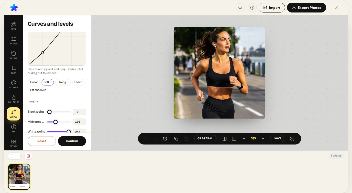
2. Levels vs. Curves: Core Distinctions and Applications
Many photographers conflate Levels and Curves. While both operate upon the luminance distribution, their mechanics serve complementary photographic roles:
The Levels Tool: Linear Anchoring and Midtone Gamma
The Levels tool operates through three primary boundary sliders: the Black Point, the White Point, and the Midtone Gamma. Its primary purpose is linear dynamic range expansion:
If a photograph captured in heavy fog or diffuse flat light concentrates all its pixels between values 35 and 215, it appears washed out and devoid of punch. By dragging the Black Point slider to 35 and the White Point to 215, the algorithm remaps this truncated range to span the full 0 to 255 scale. The Midtone Gamma slider acts as a power-law exponent (y = x^(1/γ)), brightening or darkening midtones without shifting the anchored black and white limits.
The Curves Tool: Non-Linear Multipoint Sculpting
While Levels applies a rigid linear or exponential formula across the entire histogram, Curves provides non-linear multipoint control. You can anchor deep shadows so they remain rock solid, lift upper midtones to add radiance to a model's face, and simultaneously compress specular highlights to preserve cloud details — all within a single curve using independent spline nodes.
3. The Classic S-Curve: The Secret to Natural Contrast
The most celebrated curve geometry in photographic history is the S-Curve. Almost every image that viewers intuitively perceive as crisp, three-dimensional, and professional exhibits a tonal transfer profile conforming to this sigmoidal shape.
To construct a classic S-Curve, place two primary control nodes along the neutral diagonal:
- Shadow Node (approximately at input coordinate 64): Pull this node gently downward (into the output range between 50 and 56). This anchors deep shadows, imparting physical weight and density to darker scene elements.
- Highlight Node (approximately at input coordinate 192): Lift this node proportionally upward (into the output range between 200 and 208). This illuminates highlights and injects brilliance into the frame.
Notice the resulting geometry: the central segment of the curve (governing midtones between 64 and 192, where essential facial and texture data reside) becomes significantly steeper. As established in section one, a steeper slope corresponds to higher local contrast. Concurrently, the extremities of the curve (shadows below 30 and highlights above 225) taper smoothly into gradual roll-offs, preventing blacks from blocking into empty voids and highlights from clipping into blown white.
4. Film Emulation Aesthetics: Lifted Blacks and Soft Shoulders
Over recent decades, editorial and fashion photography popularized the matte analog film aesthetic (often termed the faded film look). This look emulates the sensitometric response of chemical silver halide emulsions, where minimum optical density (D-min) was never completely pitch-black.
In PhotoEditor.sbs, you can recreate this timeless aesthetic with two precise curve interventions:
- Lifting the Black Point (Matte / Faded Shadows): Select the bottom-left anchor node (originally located at 0, 0) and drag it vertically upward until reaching an output value between 25 and 40. Now, no pixel in the final image will measure zero; the deepest shadows take on a velvety, creamy charcoal-gray appearance, stripping away clinical digital harshness.
- Highlight Compression (Soft Shoulder Roll-Off): Select the top-right anchor node (originally at 255, 255) and lower it slightly to an output value between 235 and 245. This prevents specular reflections on fabric or skin from glaring with harsh plastic intensity, recreating the organic highlight rolloff of classic color negative stocks like Kodak Portra or Fuji Pro 400H.
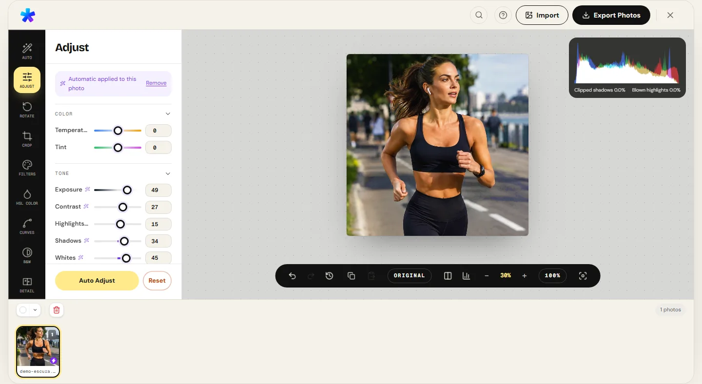
5. Auto Levels and Percentile Histogram Analysis
Clicking Auto Levels in PhotoEditor.sbs does not apply a rigid, arbitrary preset. Instead, it executes an empirical statistical analysis over the image decoded into browser memory:
- Luminance Histogram Binning: The engine samples pixel values across the canvas and compiles a 256-bin histogram using ITU-R BT.709 perceptual luminance weighting: Y = 0.2126 R + 0.7152 G + 0.0722 B.
- Percentile Anchoring (P0.5 and P99.5): Rather than keying off the absolute minimum and maximum values in the file (which often represent dead sensor pixels or rogue hot spots), the algorithm discards the extreme 0.5% of shadow outliers and 0.5% of highlight outliers.
- Dynamic Anchor Stretching: The Black Point is anchored at P0.5 and the White Point at P99.5. The active dynamic range of the scene is stretched to fill the full 0 to 255 scale without risking accidental clipping of valuable visual detail.
6. Comparative Curve Profile Recipe Table
The table below summarizes node placements and photographic effects across primary studio curve configurations:
| Curve Profile | Node Coordinates (Input → Output) | Mathematical Behavior | Visual Impact in Photography |
|---|---|---|---|
| Soft S-Curve | Shadows: (64 → 52) | Highlights: (192 → 204) | Increases derivative f'(x) in midtones while keeping endpoints locked. | Balanced contrast and three-dimensional pop without sacrificing fine textures. |
| Hard S-Curve | Shadows: (64 → 40) | Highlights: (192 → 216) | Aggressive midtone slope with rapid terminal compression. | Dramatic high-impact editorial grade for male portraits and urban architecture. |
| Faded / Matte Film | Black Point: (0 → 32) | Shadows: (64 → 68) | Vertical baseline elevation eliminating pure digital zero from the frame. | Velvety, milky blacks and nostalgic cinematic analog film atmosphere. |
| Shadow Recovery | Shadows: (48 → 72) | Midtones: (128 → 140) | Lifts lower half of the curve without modifying the 255 white point. | Brightens backlit subjects and reveals shadow detail without blowing out skies. |
| Highlight Compression | White Point: (255 → 238) | Highlights: (192 → 180) | Lowers maximum output ceiling and compresses high-key slopes. | Softens harsh glare across bright skies, clouds, and metallic reflections. |
| Reverse S-Curve (Matte Flattener) | Shadows: (64 → 76) | Highlights: (192 → 178) | Flattens central slope f'(x) < 1, compressing midtone range. | Tames extreme harsh contrast in photographs captured under midday direct sun. |
7. Technical Hazards: Avoiding the Comb Histogram and Banding
Aggressive curve and level adjustments on standard 8-bit JPEG files require disciplined technical control. Because an 8-bit file possesses only 256 discrete bins per channel, pushing curves too far stretches the tonal distribution beyond its continuous resolution threshold.
The classic indicator of this degradation is the comb histogram, where empty gaps appear between histogram bars. In published imagery, this manifests as posterization or color banding: transitions that should appear perfectly smooth — such as evening sky gradients or soft facial skin tones — fracture into noticeable concentric steps.
To prevent banding artifacts:
- Never pull shadow and highlight nodes in opposite extreme directions abruptly; maintain smooth, organic spline contours.
- Avoid extreme levels stretching on files that have already undergone aggressive JPEG compression in budget smartphone sensors.
- If a scene requires extensive contrast boosts, combine a moderate curve with subtle adjustments in the basic exposure and contrast panels.
Open the Curves and Levels tool in PhotoEditor.sbs
Open the Curves and Levels tool in PhotoEditor.sbs8. Frequently Asked Questions
Frequently asked questions
What is the fundamental difference between the Contrast slider and the Curves panel?
The Contrast slider pushes dark tones downward and light tones upward linearly around a fixed center point. The Curves panel gives you complete freedom to sculpt the transfer function, creating asymmetrical curves where you can deepen shadows without clipping highlights.
What does the 45-degree diagonal line represent in the curve graph?
The 45-degree diagonal represents the neutral baseline where output equals input (f(x) = x). Placing a point above the diagonal brightens that specific tone; pulling it below darkens it.
How do I create a faded matte vintage film look using curves?
Simply drag the bottom-left anchor point (the black point at 0, 0) upward to an output value between 25 and 35. This eliminates pure digital zero, transforming dark shadows into creamy, velvety charcoal-gray tones.
What happens when I slide the White Point marker to the left in the Levels panel?
Moving the White Point to the left (e.g., from 255 to 210) remaps any pixel with an intensity of 210 or higher as pure white (255), expanding dynamic range and brightening the overall image.
How does the Auto Levels algorithm compute adjustments?
The engine analyzes the photo's perceptual luminance histogram in browser memory, ignores the extreme 0.5% of noise pixels in shadows and highlights, and stretches the black and white points to fill the full 0 to 255 tonal spectrum.
Does adjusting tone curves alter colors in my photograph?
Yes. In standard RGB color workflows, steepening midtone contrast naturally elevates perceptual color saturation in those zones. If colors appear overly saturated following curve adjustments, gently ease back saturation in the basic adjustments or HSL panel.
Does PhotoEditor.sbs upload my photos to cloud servers to calculate curves?
No. All cubic spline calculations, histogram binning, and real-time canvas rendering execute 100% locally on your computer via TypedArrays and the HTML5 Canvas API. Your files remain completely confidential.
What formats are available to save my photo after curve adjustments?
You can export your finished photograph in high-quality JPEG with adjustable compression, in PNG for uncompressed color fidelity, or WEBP export (when the browser supports it) to minimize storage footprints for web delivery.