In digital photography, relying solely on your computer screen or smartphone display to judge whether a photo is properly exposed is one of the most perilous traps. Human visual perception is heavily swayed by ambient room lighting, direct sun glare reflecting off glass screens, and the device's own automatic brightness settings. An image that appears clean in a dim room can turn out muddy, crushed, and severely underexposed when evaluated on a calibrated workstation monitor or sent to physical print.
The only objective, mathematically infallible tool immune to optical illusions is the histogram. A histogram translates every single pixel in your photograph into a live statistical frequency graph of brightness distribution. In this comprehensive technical guide, we break down the anatomy of 256 luminance levels, the irreversible consequences of shadow and highlight clipping, reading individual RGB color channels, comb-like quantization artifacts, and how to sculpt your histogram using PhotoEditor.sbs's Curves and Levels and Adjust Photo tools — running 100% locally in your browser.
1. What Is a Histogram: The Mathematical X-Ray of Light
In computer imaging, a histogram is a continuous bar chart displaying the statistical frequency of each discrete brightness value recorded across your image:
- The horizontal axis (X) maps brightness, spanning from pure digital black on the far left (level 0) to pure digital white on the far right (level 255 in standard 8-bit imaging).
- The vertical axis (Y) represents the total population count of pixels in your photograph that share that exact luminance coordinate. Tall peaks indicate heavy pixel clustering at that specific tonal band; low troughs indicate sparse representation.
There is no universally "correct" histogram shape. A high-contrast sunset silhouette will naturally group pixels at the opposing polar extremes, whereas a soft morning fog capture will cluster its data into a slender mountain right in the midtones. An editor's goal is not to force an artificial bell curve onto every frame, but rather to guarantee that the tonal spread honors the artistic intent without discarding critical detail through boundary clipping.
2. The Five Tonal Zones Across the Horizontal Axis (0 to 255)
To read a histogram with professional proficiency, segment the 256-level horizontal continuum into five functional reference zones:
1. Deep Blacks (Levels 0 – 15)
The foundation of true blacks. Reserved for elements requiring zero interior texture — such as deep rock fissures, dark pupils of the eyes, or the void of open night sky.
2. Textured Shadows (Levels 16 – 64)
The region housing delicate folds in dark fabrics, tree bark, and dark hair. Crushing this zone down into pure black strips an image of its organic tactile realism.
3. Midtones (Levels 65 – 190)
The perceptual centerpiece of photography: encompasses human skin, architecture, green foliage, and everyday surfaces. The human retina exhibits its highest discrimination for subtle gradients here.
4. Textured Highlights & Whites (Levels 191 – 255)
From levels 191 to 245 sit bright textured surfaces (sunlit clouds, white garments, beach sand). From 246 to 255 reside specular glints and raw reflections off water or polished chrome.
3. Shadow and Highlight Clipping: The Point of No Return
The most severe irreversible technical failure in digital photography is clipping. Clipping occurs whenever scene brightness exceeds the physical storage boundaries of the digital image format:
- Shadow Clipping (Crushing): Occurs when the left slope of the histogram collides with the vertical wall at level 0, stacking upward into a vertical spike. Every pixel caught in that spike loses all textural nuance, converting into flat, featureless solid black.
- Highlight Clipping (Blowing): Occurs when pixel luminance exceeds the digital ceiling and crashes into the right vertical wall at level 255. Cloud textures, skin highlights, or wedding dress lace become totally obliterated into pure, unrecoverable white paper.
4. Luminance Histogram vs. Individual RGB Color Channels
Many novice retouchers monitor only the global gray luminance histogram while ignoring separate Red (R), Green (G), and Blue (B) channel histograms. That oversight often ruins colorful compositions:
Consider a vibrant close-up photograph of a bright red rose petal. The combined gray luminance curve may appear comfortable and centered, nowhere near the 255 right border. However, inspecting the dedicated Red channel reveals that red pixels are slammed hard against the right wall. This is known as chromatic channel blowout: the petal loses all textural veins, collapsing into a flat, glowing neon blotch devoid of three-dimensional depth.
5. The 'Comb-like' Effect and Digital Posterization
When applying extreme contrast corrections — dragging curve and level endpoints aggressively on standard pre-compressed 8-bit rasters —, you may notice narrow, empty vertical gaps appearing across your histogram like the teeth of a comb.
This artifact signals digital quantization error: the source file lacked sufficient intermediate color gradations to populate the stretched dynamic range, forcing the rendering engine to skip integer steps. Visually, this manifests across the image as visible stair-stepped banding across smooth skies and portraits, known throughout the industry as posterization.
6. Diagnostic Reference: Histogram Shapes and Solutions
The diagnostic table below matches classic histogram profiles with underlying photographic causes and corrective actions:
| Histogram Profile | Photographic Diagnosis | Visual Scene Impact | Corrective Action & Tool |
|---|---|---|---|
| Mass stacked on the far left (crashing at 0) | Severe underexposure with shadow crushing | Opaque shadows, dark faces, lost texture | Increase Exposure (/adjust-photo) and lift black level |
| Mass stacked on the far right (crashing at 255) | Severe overexposure with highlight blowout | Blown-out skies, chalky skin highlights | Lower Exposure and pull down highlight ceiling |
| Narrow hump huddled purely in center | Low dynamic contrast (flat foggy scene) | Dull, lifeless, gray wash lacking punch | Apply an S-curve (/photo-curves) to stretch endpoints |
| Two tall polar spikes with a deep valley | High dynamic range (harsh direct noon sun) | Simultaneous pitch-black shadows and harsh glares | Compress tonal range with a gentle reverse curve |
| Red channel pinned flat against right border | Chromatic saturation blowout in warm hues | Petals or car paint lose all fine texture | Reduce red saturation (/adjust-photo) |
7. Step-by-Step: Sculpting Histograms in PhotoEditor.sbs
PhotoEditor.sbs computes 256-bin histogram distributions in real time within your browser memory, enabling responsive interactive tonal shaping:
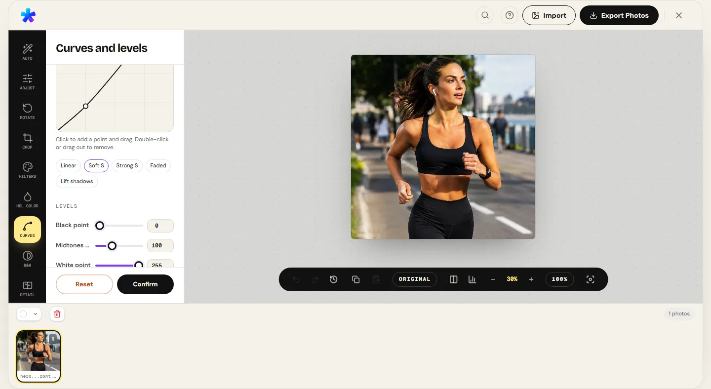
Step 1: Open the Curves and Levels Tool
Navigate to Curves and Levels and load your original photograph.
Step 2: Inspect Tonal Endpoints
Examine the histogram underlay behind the curve grid. If an empty gap exists between the left border and the beginning of the pixel mountain, gently drag the black point input handle inward until it meets the first pixels.
Step 3: Sculpt Contrast with an S-Curve
Click the center of the diagonal line to establish an anchor point for your midtones. Place a second node along the upper-right quadrant and drag slightly upward to brighten highlights; place a third node along the lower-left quadrant and drag downward to enrich shadows — creating an authentic tonal S-curve.
Step 4: Verify Color Balance in Adjust Photo
Switch to Adjust Photo to verify that no individual primary color channel is pinned against extreme borders.
Honest Technical Boundary Note
The histogram inside PhotoEditor.sbs computes statistical 8-bit-per-channel luminance and RGB bin counts directly from the rendered image pixels in the browser Canvas. It operates as a rendered-state histogram display, rather than an un-demosaiced linear raw sensor photodiode meter.
Open Curves and Histogram in the Editor Now
Open Curves and Histogram in the Editor Now8. Frequently Asked Questions
Frequently asked questions
What does it mean when the histogram line crashes into the right edge?
It indicates highlight clipping. Pixels in that area exceeded digital level 255 and collapsed into pure solid white with zero recoverable textural detail.
Is there a perfect bell-curve histogram shape that all good photos must follow?
No. A histogram should reflect the authentic lighting of the scene. A snowy mountain photo naturally concentrates pixels toward the right, while a night cityscape groups pixels on the left.
Why does the histogram on my camera LCD differ from the editor's histogram?
Cameras typically generate their on-screen histogram from an internal, pre-rendered preview JPEG that applies the camera manufacturer's proprietary contrast and picture profile.
Does PhotoEditor.sbs charge fees for inspecting or manipulating histograms?
No. PhotoEditor.sbs is completely free. There are no subscriptions, no locked features, and no watermarks placed on exported photos.
What is an S-curve and how does it reshape the histogram?
An S-curve lifts highlights while pulling down shadows, expanding the distance between histogram peaks to deliver greater perceived contrast, depth, and clarity.
Will my photograph degrade when adjusting curves and levels?
Moderate adjustments cause no visible degradation. However, extreme tonal stretching on 8-bit files can cause comb-like gaps and banding artifacts across smooth skies.
Does analyzing histograms consume cellular internet bandwidth?
No. All 256-level histogram bins, mathematical curve splines, and pixel calculations run 100% locally on your computer or mobile device within the browser.
What image formats are available when saving my calibrated photograph?
You can export your completed photo in high-quality JPEG or lossless PNG, as well as in WebP format when the browser supports Canvas WebP encoding.